CQL Demo
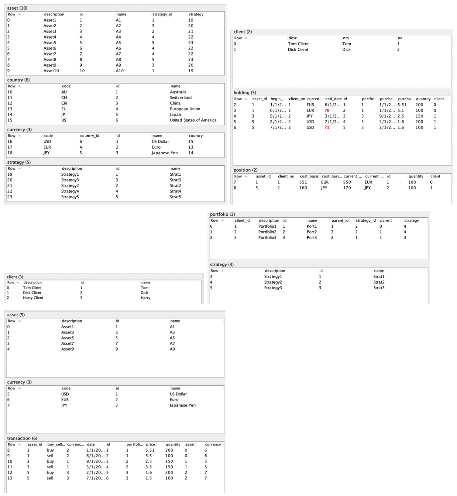
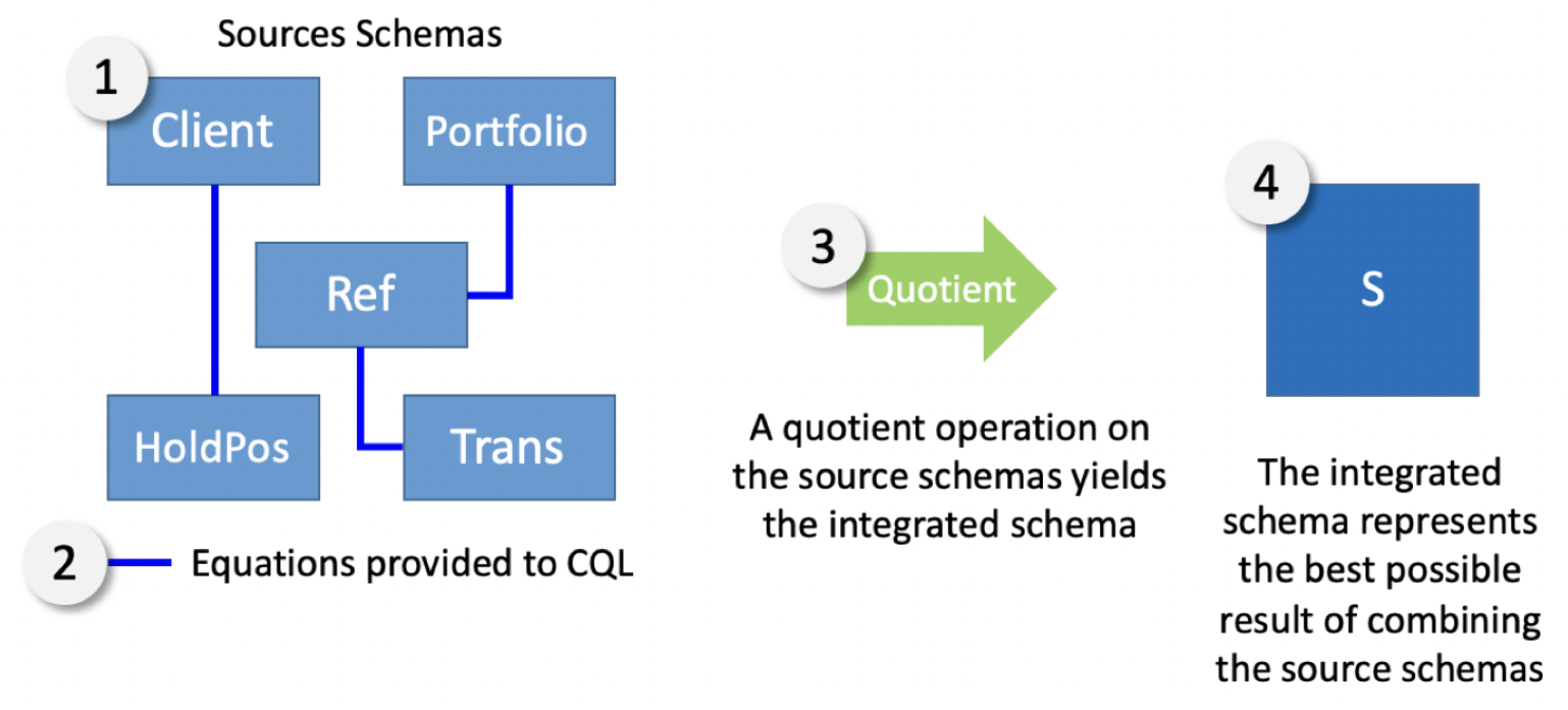
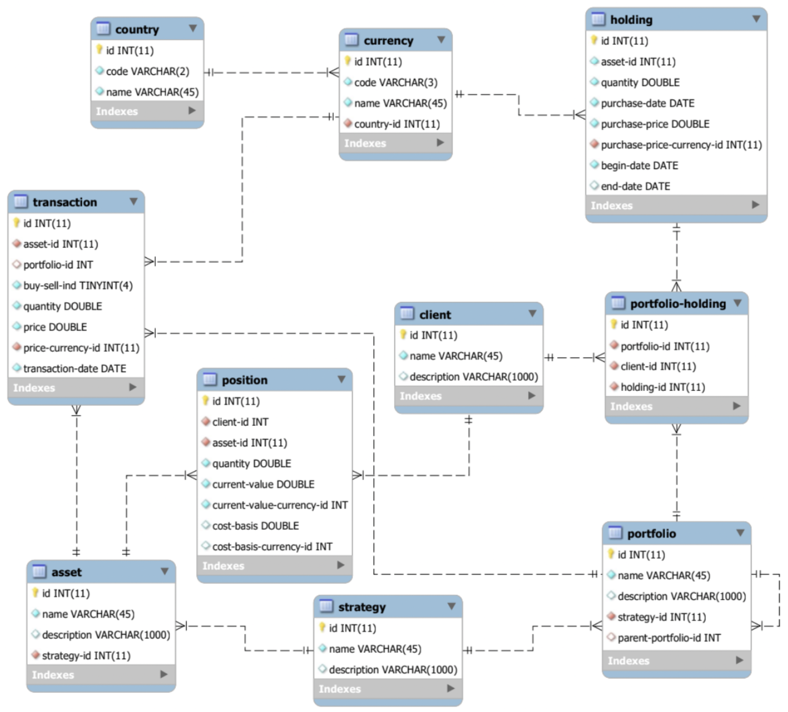
To demonstrate this rapid schema and data integration capability in CQL we will walk through an example (based on the built-in ‘FinanceColim1’ example) of integrating a typical collection of systems for investment management. Because they were built or acquired as separate systems, they contain redundant data whose format and completeness may not be consistent and whose relationships are unclear. Some of the data will come from CSV files on my local computer, some of the data will come from an SQL database on a remote AWS server, and some of the data will come from typing it into CQL directly. The data make up five independent databases, like this:
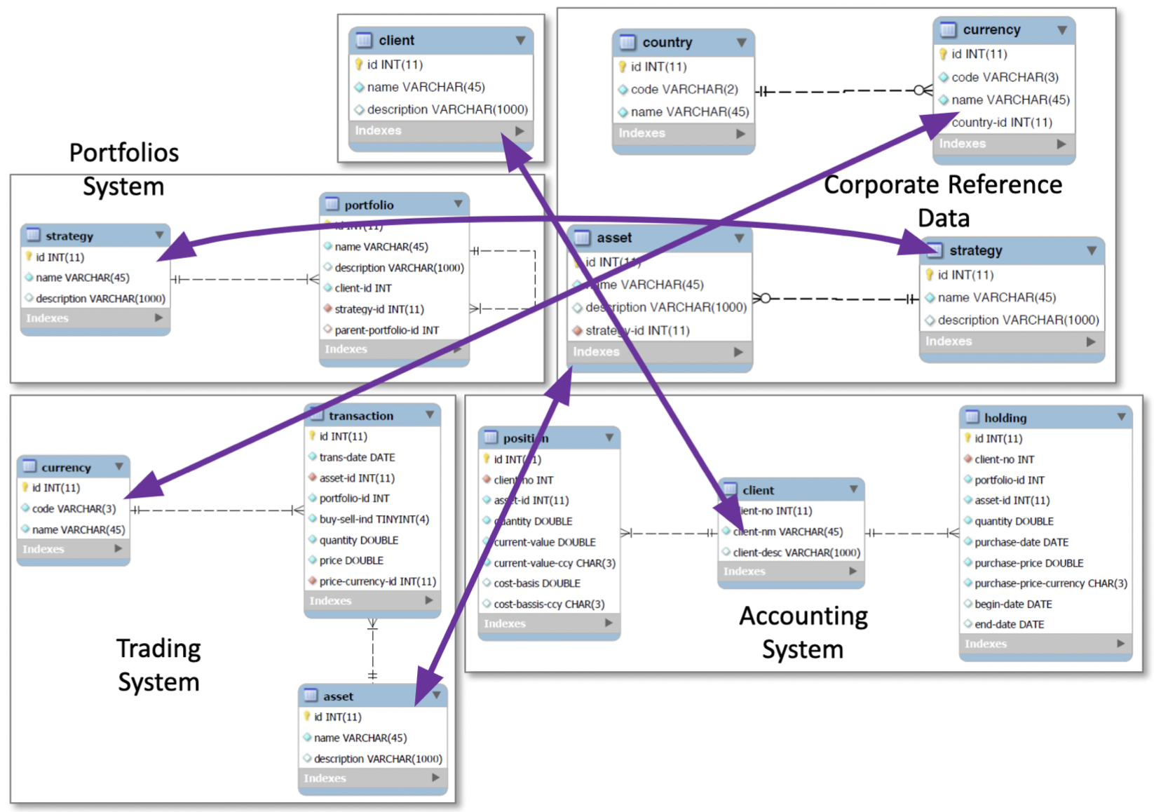
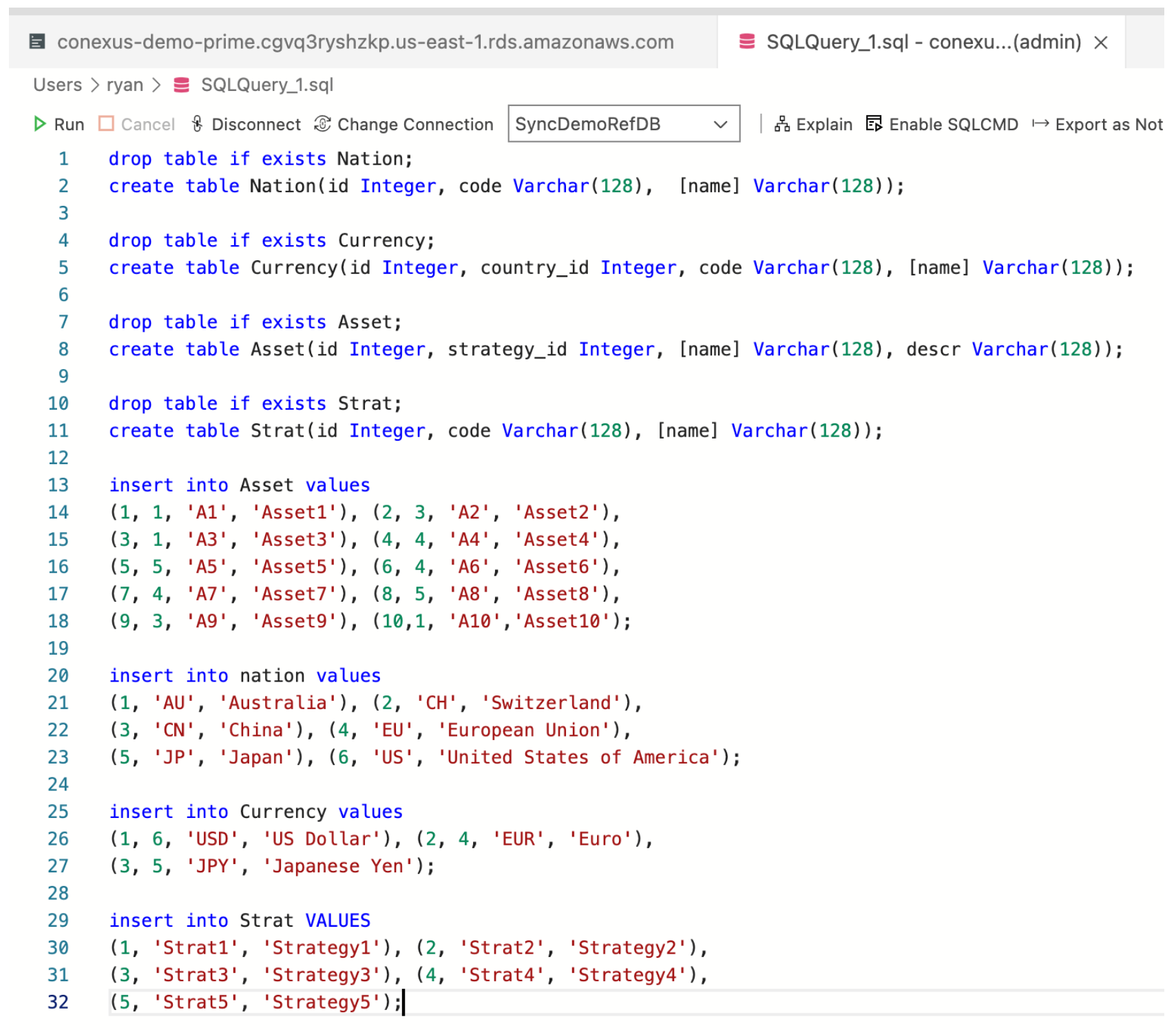
Although the diagram draws foreign key lines, there is no requirement that source data contain foreign keys. And in fact, as we will see, the actual SQL databases used in this demo contain no key declarations at all, primary or foreign. The source data is displayed in CQL below for reference.
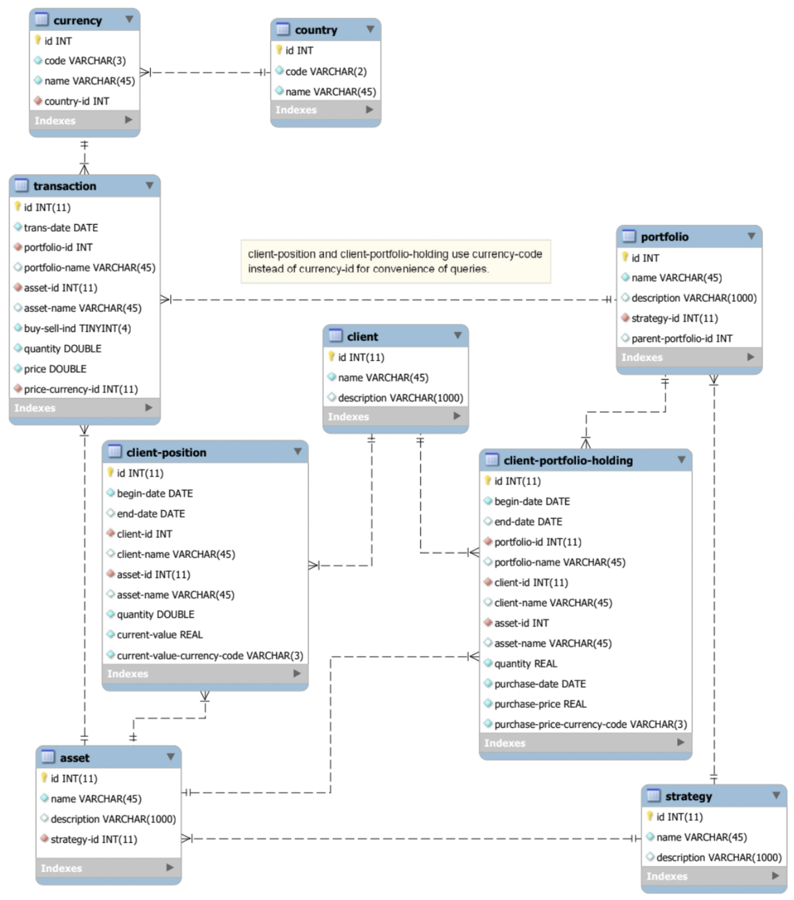
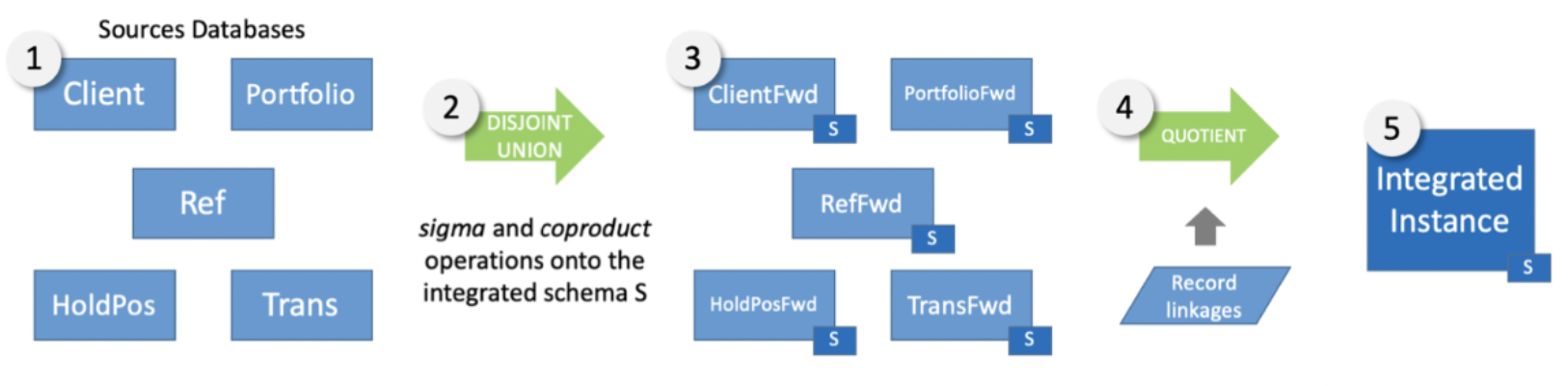
Our goal is to integrate the data onto a new integrated schema, to be stored in a data warehouse (e.g. Snowflake):
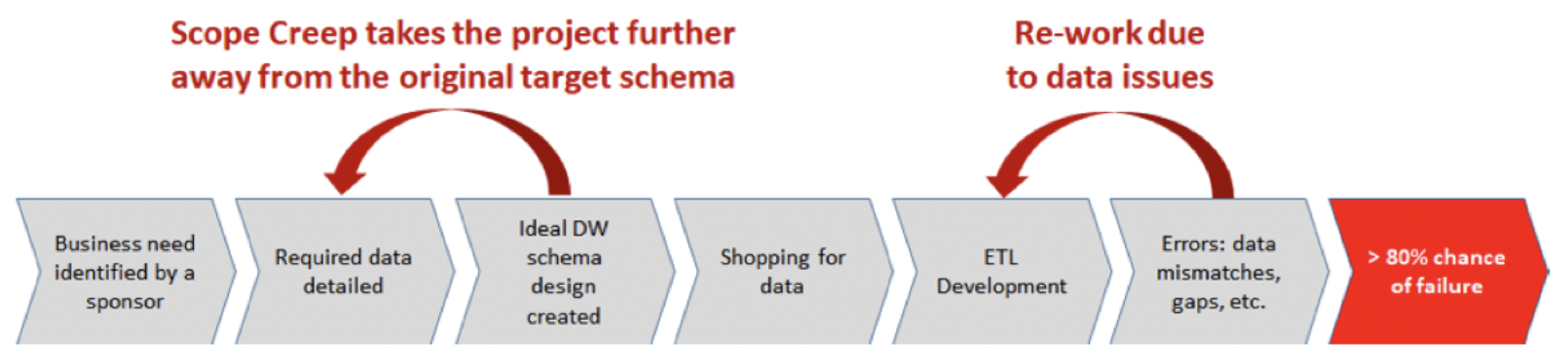
Today, the data warehousing problem described above is solved in SQL, Informatica, etc., by having developers write (or rather, guess) code or schema mappings, run them, load the warehouse, see if anything breaks and/or the report/analysis seems “reasonable”. This process is not only costly, error prone, informal, and hard to automate, but requires running potentially large queries on potentially large datasets — not something that is always feasible. The traditional warehousing process is done backwards, because it starts with reporting requirements which in turn drive the warehouse schema design, which may or may not be constructible by the available data.
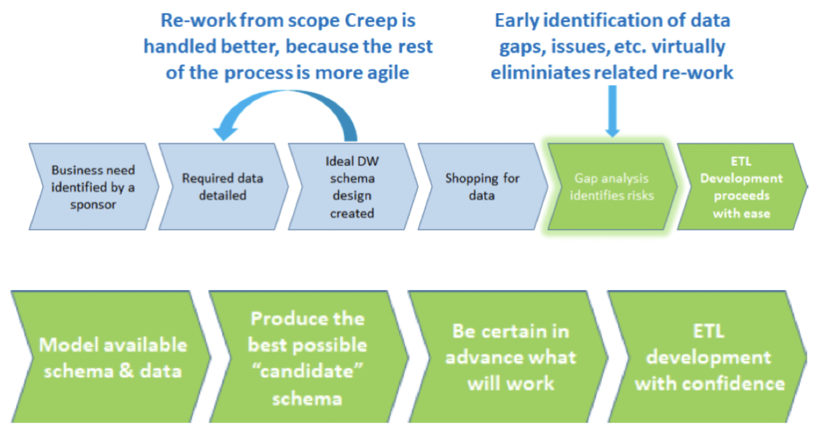
Learning from the mistakes of the backwards methodology, and using mathematics, the CQL approach implements the same warehouse in a forward way, as a function of the source schemas rather than the target. Rather than attempt to directly map to the target schema, in CQL we divide the process into two parts: integrating the source schemas and data in a (unique!) universal way that does not depend on the target, and then projecting from this universal warehouse to the desired one. We will walk through both steps in detail in this demo. In particular:
- The IT team takes the source schema and uses CQL to define the relationships between the input schemas. From this specification, CQL computes the unique optimally integrated schema that takes into account all of schema matches, constraints, etc.
- The integrated schema is compared to the desired data warehouse schema to create a gap analysis that quantifies the difference between the available source data and what the project team needs. Many of the data issues are uncovered before any development begins and before any data is moved, allowing up-front risk mitigation.
- The next step is similar to the previous, but at the data level: the IT team defines the record linkages (e.g. match by primary key) between elements related across input databases, and CQL emits the unique optimally integrated data warehouse compatible with the links. This step can be performed in memory using the CQL IDE itself, or performed via code generation to back-ends such as Spark and Hadoop.
- The IT team writes a CQL query from the integrated schema to the target schema. The CQL Automated Theorem Proving AI checks, without running the query or looking at data, if any of the target data integrity constraints do not logically follow from the integrated schema constraints and query definition.
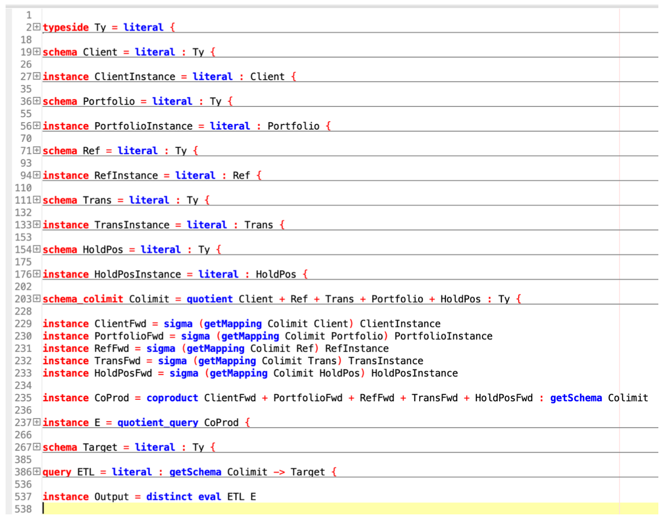
To implement the above scenario requires a total of 22 definitions, shown here folded in the CQL IDE. There are 5 source schema definitions, 1 target schema definition, 5 data import definitions, 1 schema merge definition, 1 instance merge definition, and 1 query definition. The remaining 8 definitions are formulaic scaffolding — i.e., defining names for databases to be reused later. We will walk through each of these in turn.
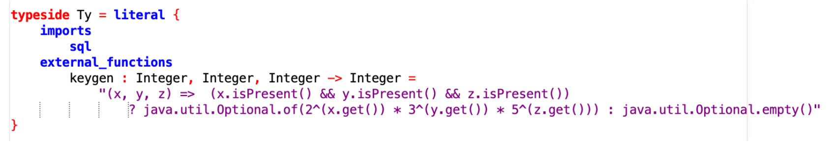
Step 1: Define the data types and user-defined functions involved
Every CQL development starts by defining the data types and user-defined functions (from any GraalVM language) that will be used in it. In this example, we will use the SQL type system, and add a key-generating function that creates unique integer keys from its three input integers — we will use it in the final step of projecting from the universal data warehouse to the desired warehouse. CQL uses Java’s Optional type for SQL’s nulls, so the keygen function can be seen manipulating the option type.
Step 2: Define the schemas for all “landed” source data sources
In general, we don’t want to import entire enterprise databases into CQL or any other tool — they won’t fit! Plus security, privacy, etc. So, like other tools, in CQL we only “land” the fragment of the source data we are interested in. For each input source database we want to land, we write a CQL schema to define the structure of the landed data, and then we write queries in the source language to actually land the data.
SQL/JDBC Import
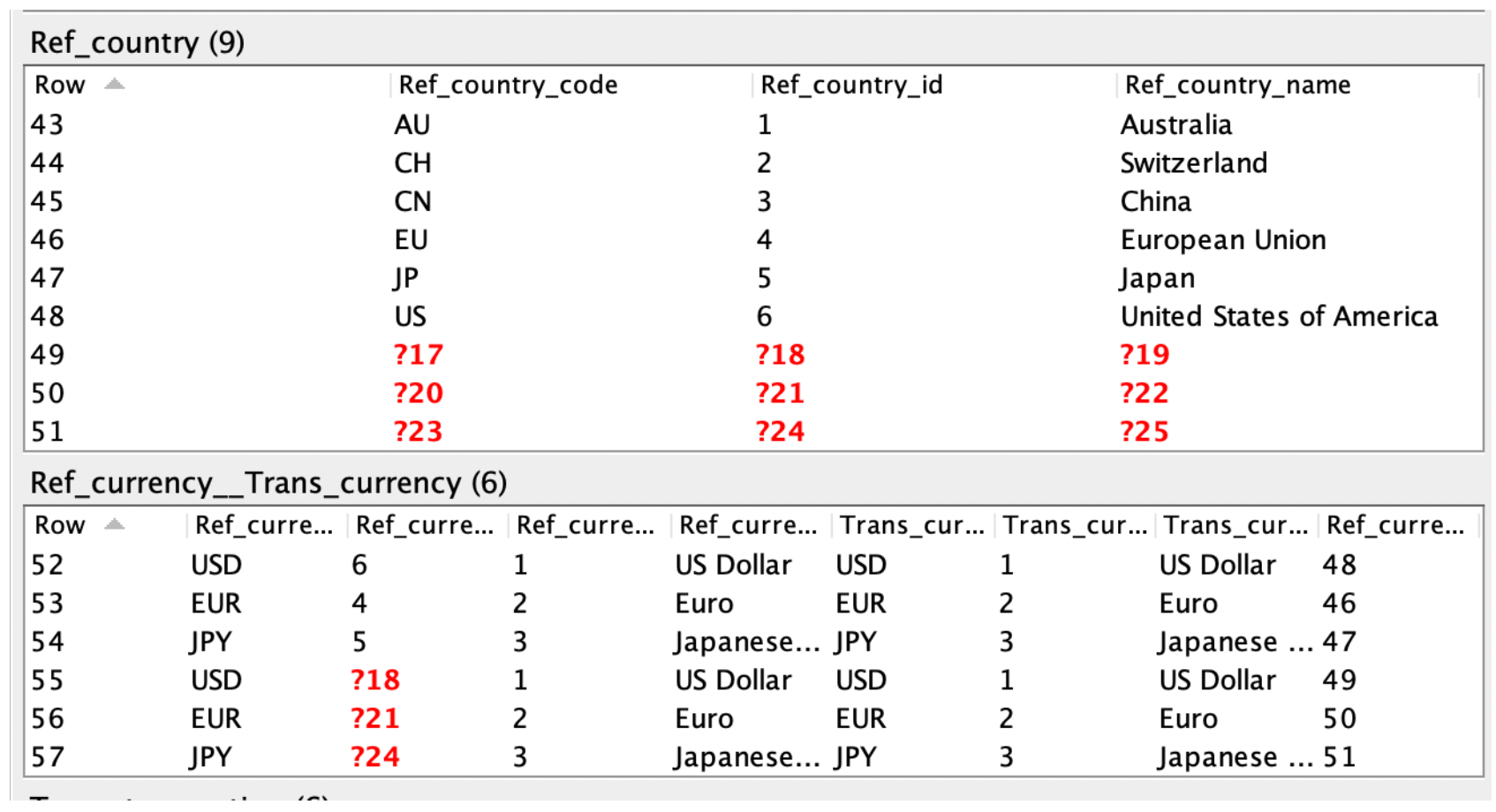
So for example, to land SQL data we write, for each CQL entity, an SQL query saying what data to land. Such SQL queries mediate between column names, change data types, hook up foreign keys, and so on. Below is shown the landing schema for the “Ref” (Reference Data) database. Note that it includes two non-trivial data integrity constraints — two foreign keys. Such constraints can be scanned for in the input data (what we do in this demo), imported from e.g. SQL automatically (a la the DUA product), inferred by AI, etc, but in practice we usually find that these constraints are in the heads of database architects, who can now formalize and store them directly in CQL.
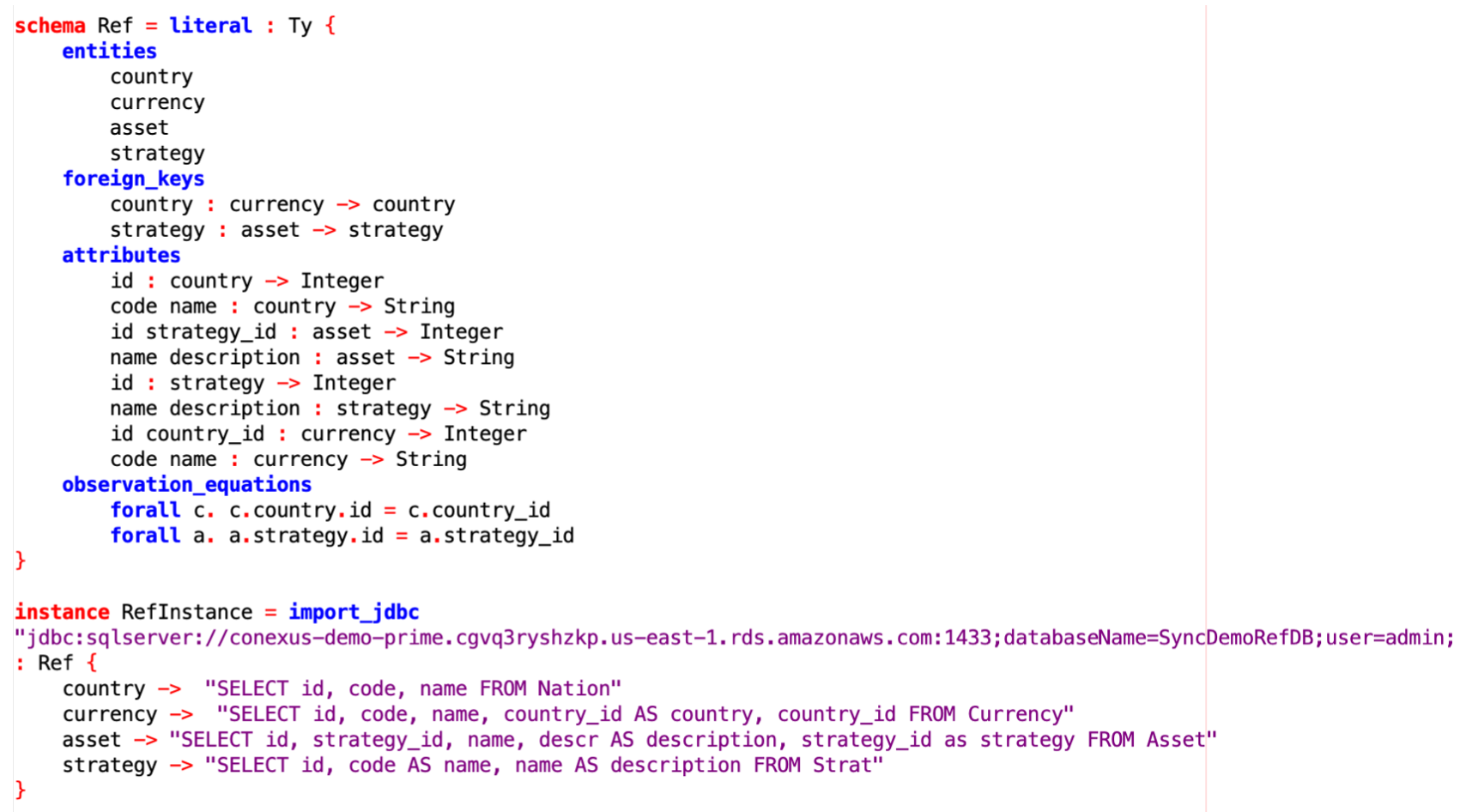
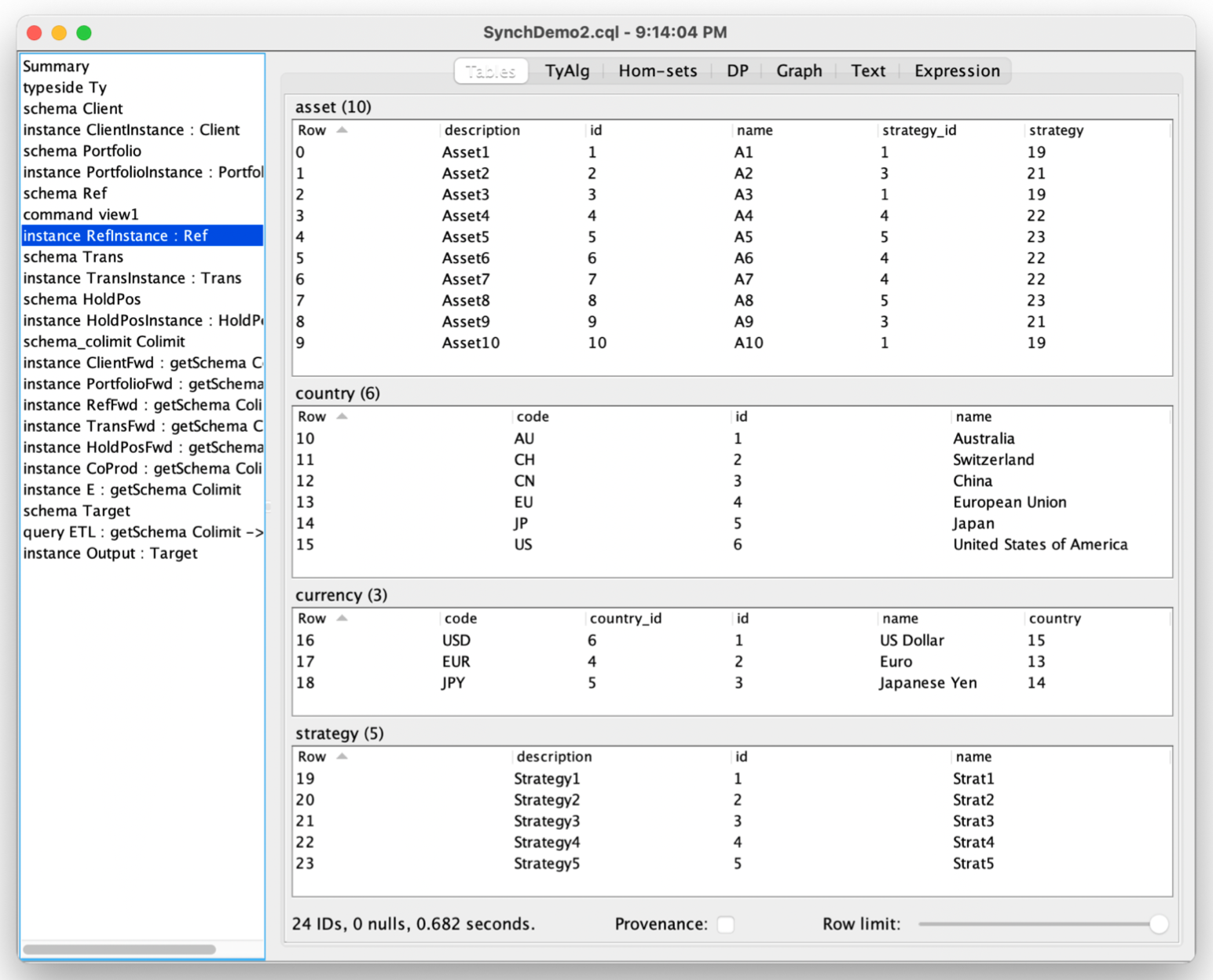
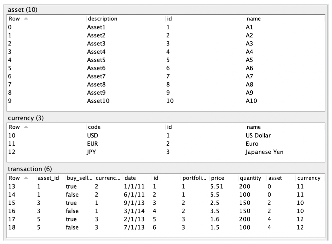
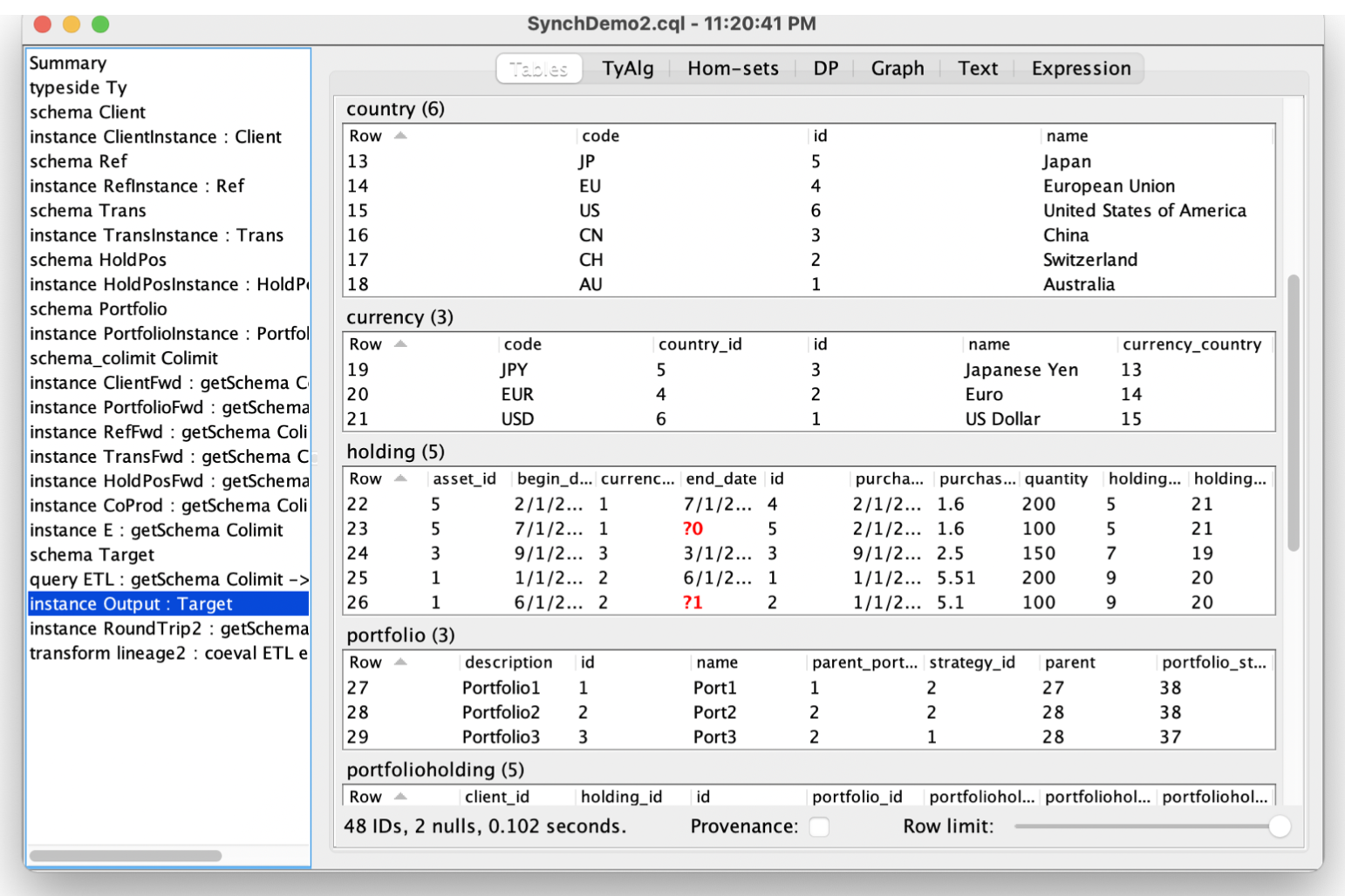
Once landed, the data may be displayed by CQL as above. Constraints are checked by CQL on load (toggleable setting); here’s an example with dirty data set to ‘halt’:

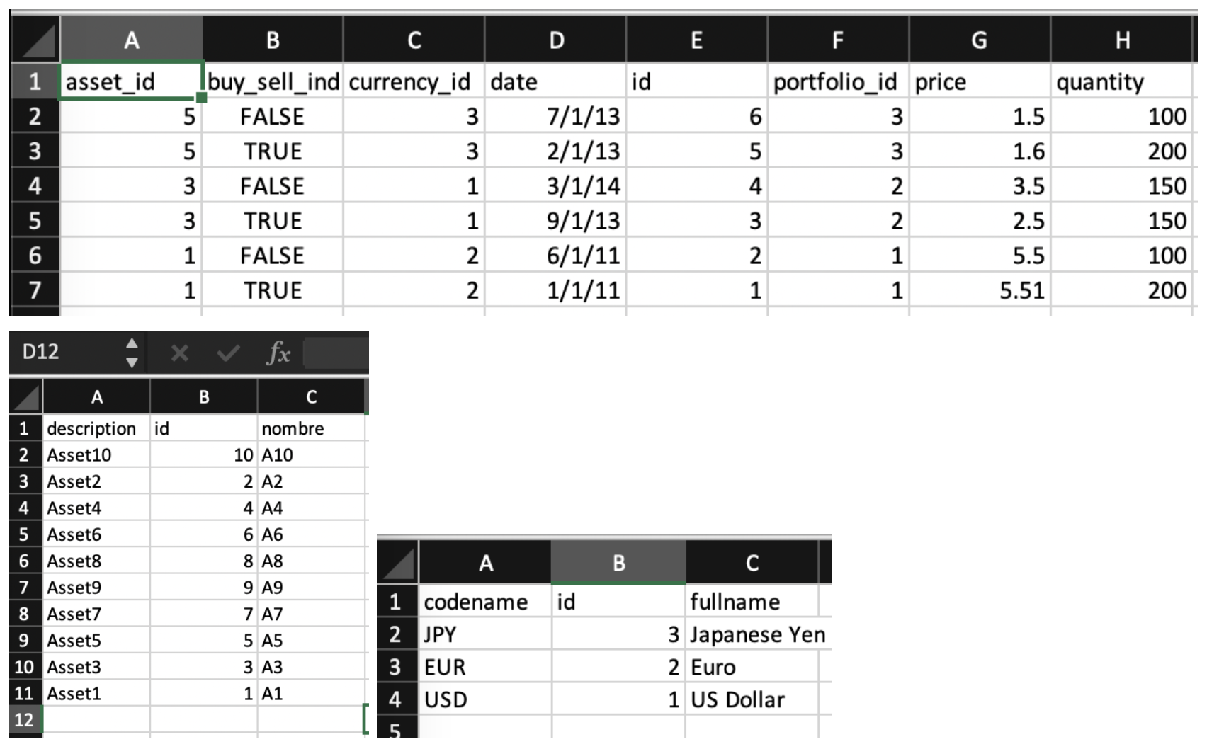
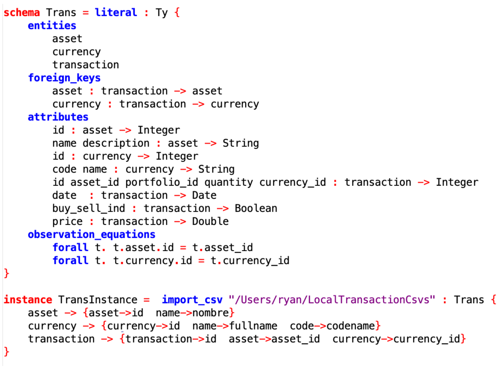
CSV Import
Similar to SQL/JDBC import, CSV import is a lightweight version of SQL import, where column names can be remapped; for more complex transformations, the recommendation is to import CSV data as-is and then use CQL schema mappings to perform transformation. In this example we have some column renaming as we import Transaction Data:
Step 3: Define the schema overlap for all “landed” source data sources
Having landed our source data (or having only defined the landing schemas), we proceed with schema integration. Mathematically, we disjointly union the input schemas together and then add additional equations (rules) to capture equivalent tables and columns. In general, user defined functions can appear in the rules, so we could write eg. client_name = toUpperCase(client_nm), for example. Conceptually, there is no choice in these rules — they follow from the intended meaning of the input data: e.g., no matter what our target schema is, that client_id and client_no will be equal in the source data is a business rule that everyone in the organization should in principle agree on, and much like the previous step, architects can write these rules down directly, or the rules can be inferred using ‘schema matching’ technology (such as in the SQL validator demo you saw last time).
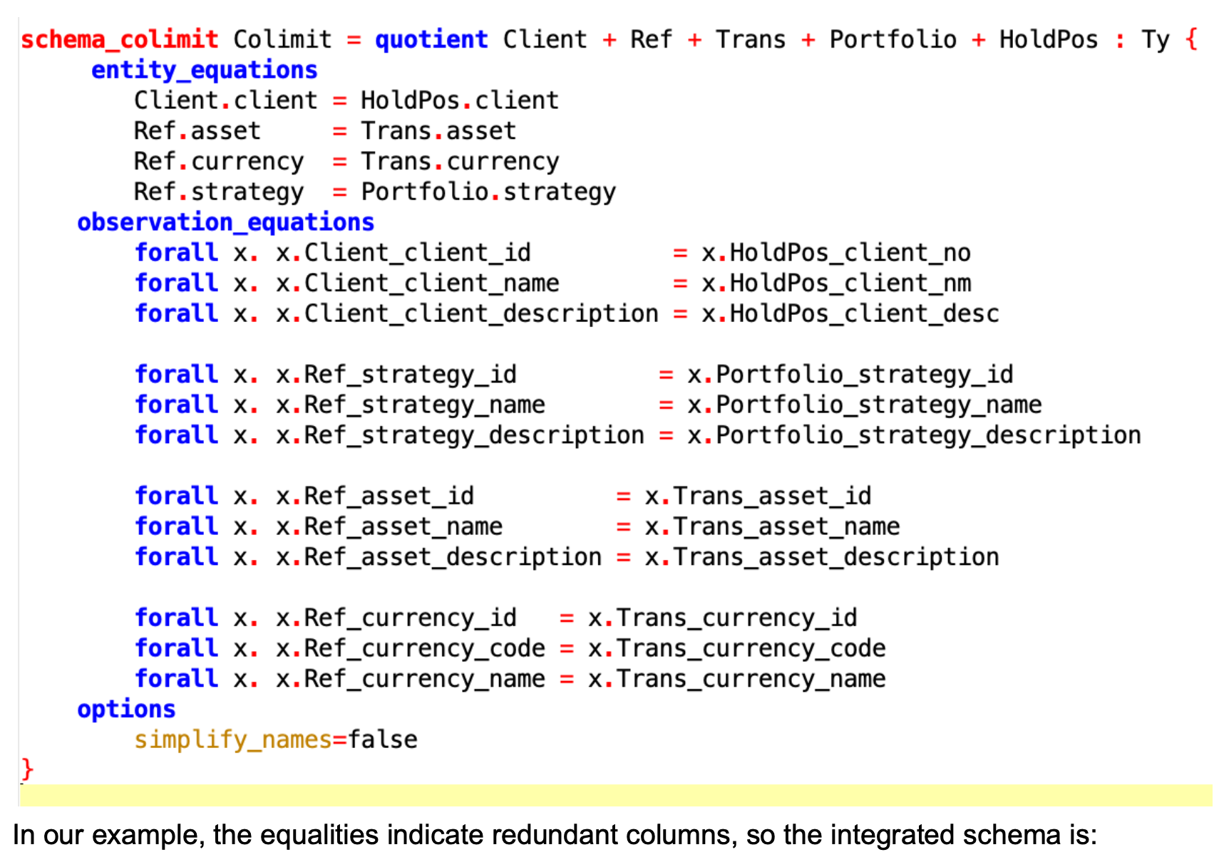
The ‘simplified’ names in the E/R diagram are precisely those we’ve disabled in the CQL code, to help illustrate simplified vs full naming in integrated schemas.
Step 4: Define the data overlap for all “landed” source data sources
With the integrated schema in hand, we can transform each landed source database onto it, and then take the disjoint union of their data with the following formulaic CQL commands (these commands will be the same for every warehouse built in the manner of this demo).
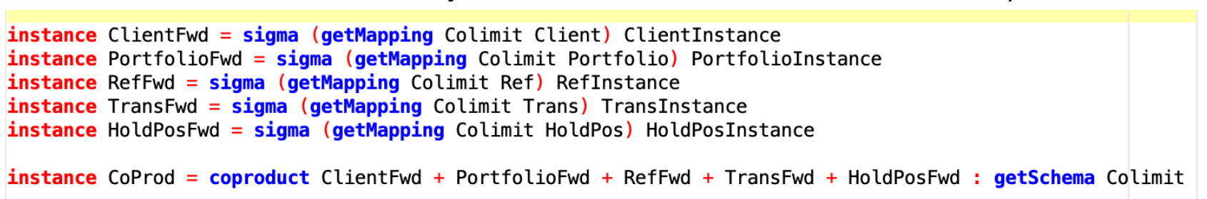
At this point we aren’t quite done — we’ve taken each landed source database, transformed it to live on the integrated schema, and then disjointly unioned them together. But we still have gaps in our data because although we have merged columns in our schema, we have not yet merged any rows in our data.
That is, during schema integration, client_id = client_no means that to answer queries about client_id one can query client_no; it does not mean that two clients that have the same client ID and number are the same client, although that is indeed desired in this example. Hence the next step, “record linking”, where we specify rules about how data is to be merged.
The schema-level rules are often a good starting point, but these rules can also be implicit in architect/programmer minds, or generated using AI techniques.
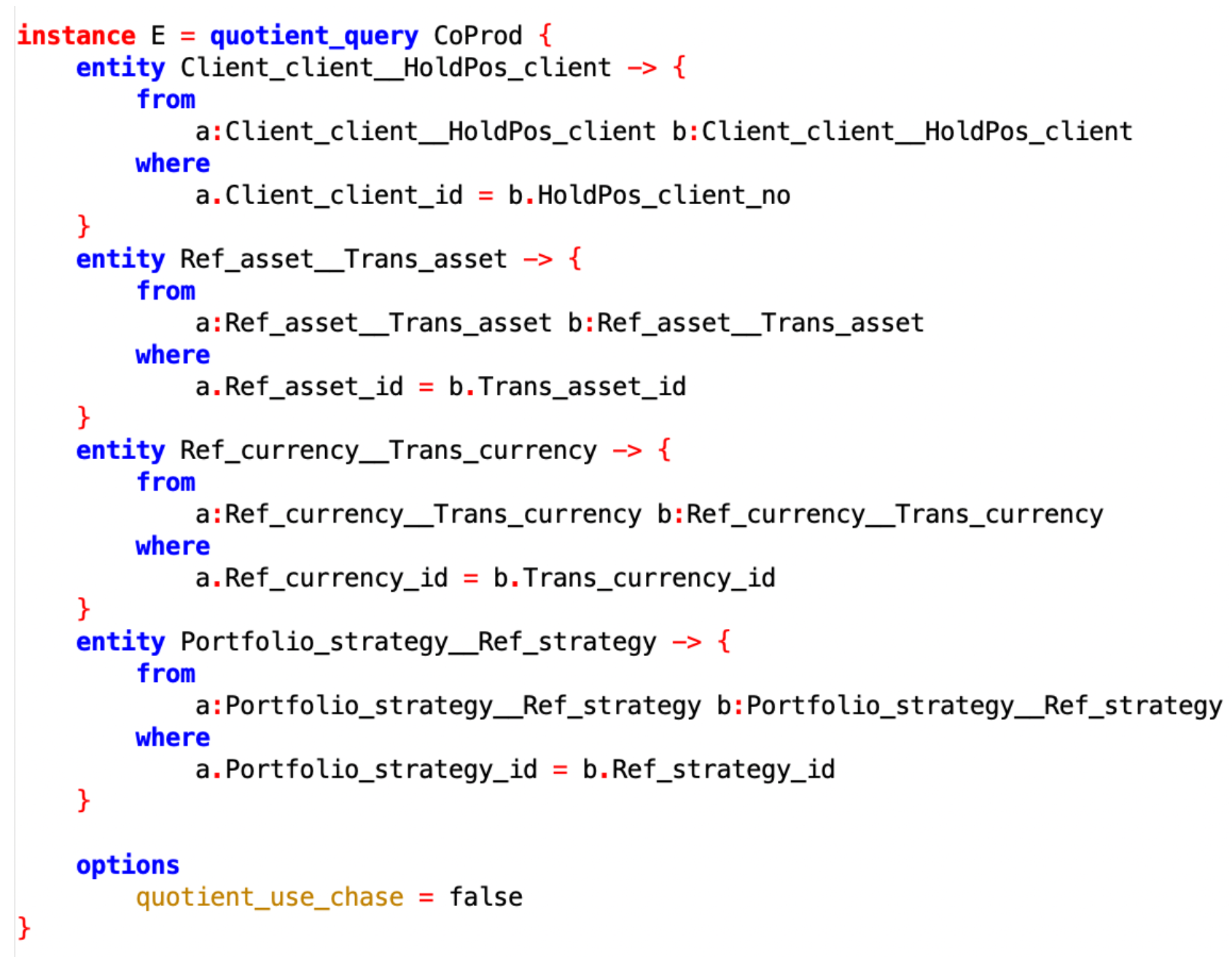
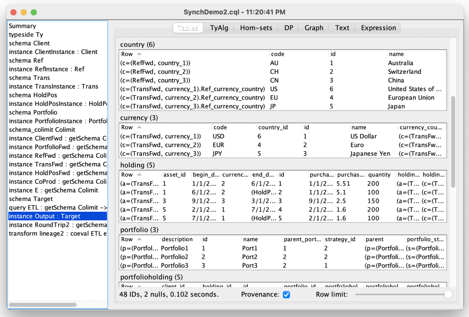
The use_chase option toggles between algorithms that are “fast for big data but slow for small data” and vice versa. We have now constructed a “universal data warehouse”, in which the missing values from before are gone:
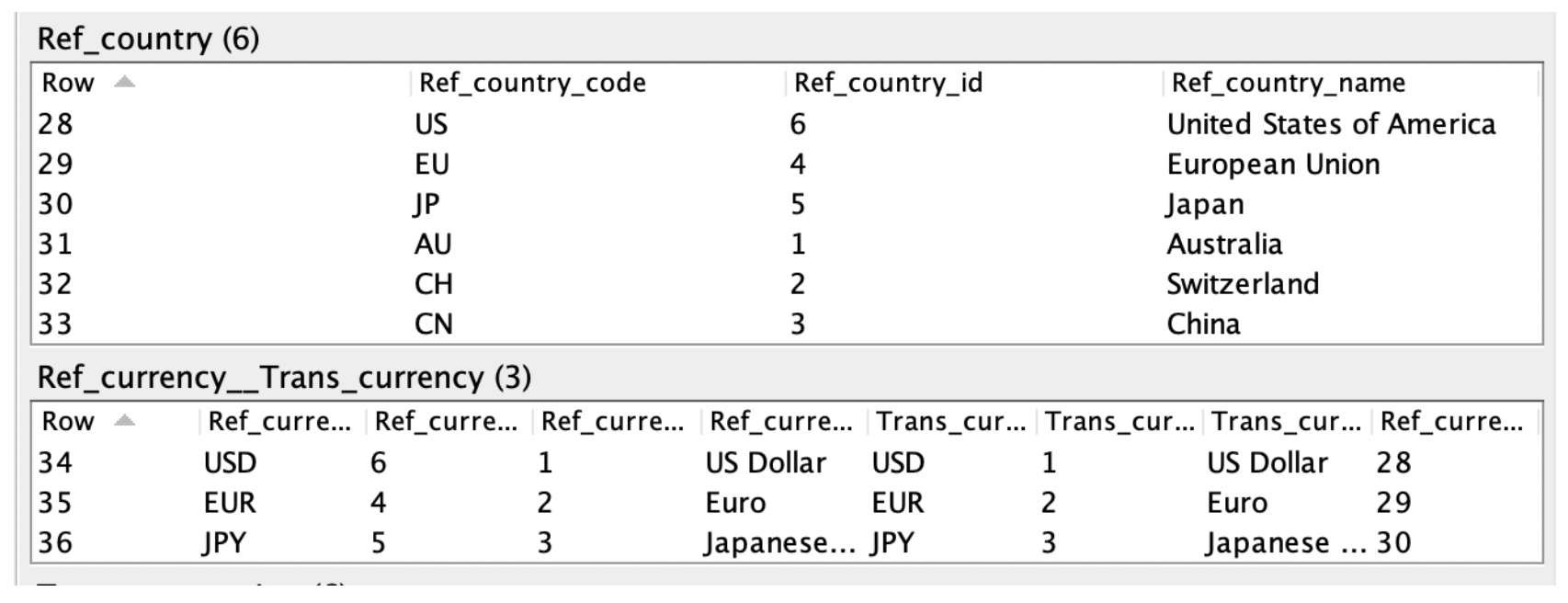
In particular, there are now 3 currencies, not 6; without a record linking step, the number of rows in the integrated database will always be the sum of the number of rows in the input, no matter how many equations are written down.
Step 5: Query the Universal Warehouse to produce the desired one
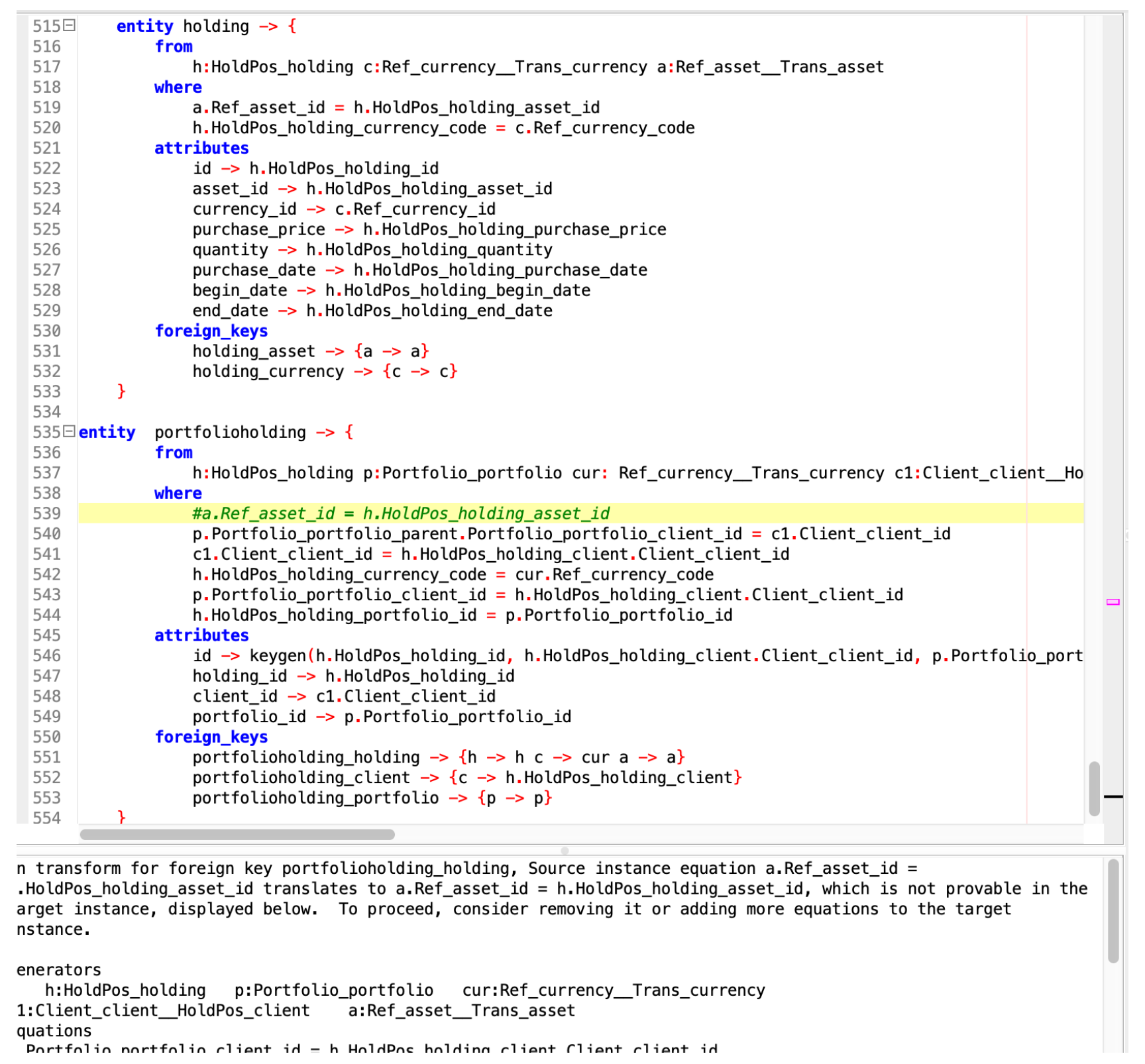
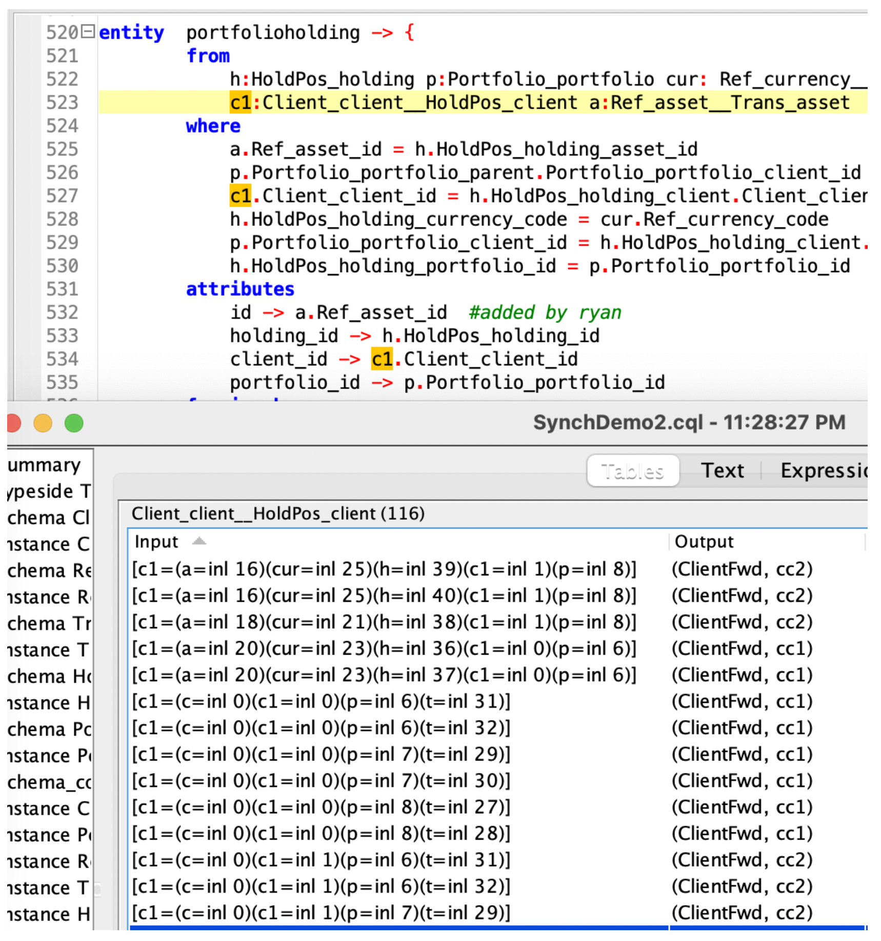
All that remains is to project from our universal data warehouse to the desired target schema. This is done using a CQL “query,” which looks a lot like a set of SQL queries equipped with additional information about how foreign keys are to be connected; CQL requires exactly one such ‘sub-query’ for each target table. CQL comes with a unique value proposition: any data integrity violations will be caught automatically at compile time by the CQL automated theorem prover AI, without running the data. In this particular example it is the portfolio holding table that is tricky to construct:
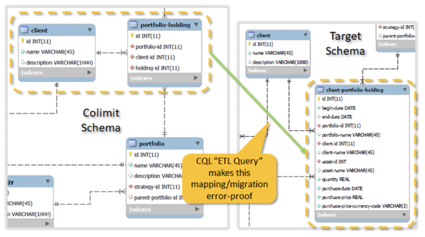
In the image below, we populate the portfolio holding table by doing a multi-way join; if we comment out one of the where conditions (in green), we see an error message from CQL.
Step 6: Load the universal data warehouse
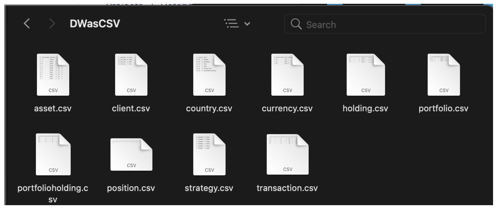
Any data model CQL can import, it can export. So for example we can eg emit this warehouse to CSV:
Provenance
Every data value constructed by CQL carries with it the full provenance of where it came from in a mathematically universal way. Here’s a screenshot of the provenance in this warehouse, where each row is showing the value of the FROM-bound variables that created it:
Round-tripping
In this example, we can perform a round-trip analysis on the universal warehouse data and query to reveal that the round-trip is surjective (because every client participates in the portfolio holding table at least once) but not injective (because some clients participate more than once, through their various holdings). The high multiplier (3 clients vs 116 client holding positions) indicates that client information is only a small part of what makes up the portfolio holding table.
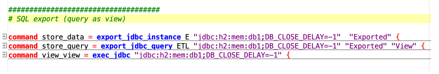
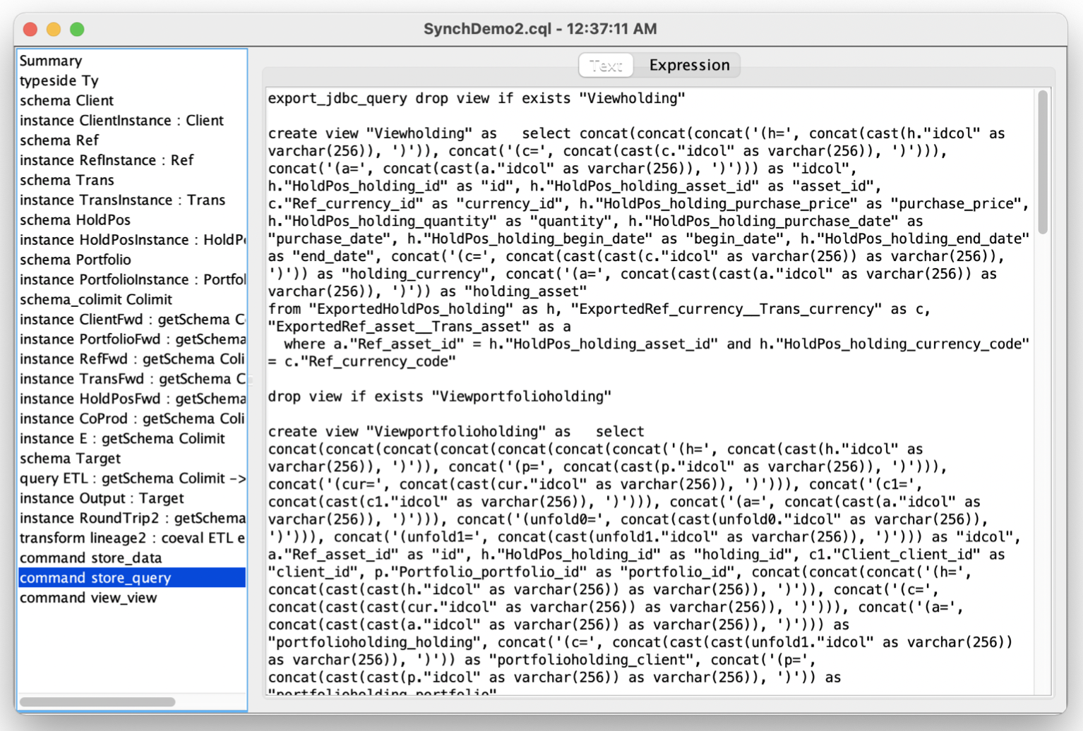
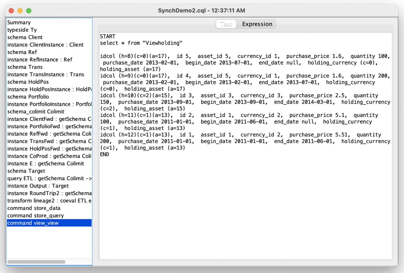
SQL Query Export
CQL queries can be exported in SQL, typically (but not necessarily) through a ‘view.’ In this example, we may export both the universal warehouse over JDBC as well as the CQL query that populates the target schema. Note that provenance is preserved in the queries- the result of listing the view shown contains not only numbers such as 5.1, but string identifiers that look like eg. “(a=2)”, a reference back to the 2nd asset in the universal warehouse.